|
The connection between factors and zeros are that factors are the factored form of zeros. For example, a zero could be x=2, but the factor would be (x-2). Division helps us factor the polynomials because it helps us break down the factors one by one. If you use synthetic division, you are also able to start with the easy zeros until you find the harder ones through the steps of division. The degree of the polynomial helps us to predict the number of zeros because that number is the amount of times that the line of the graph crosses the x axis. That doesn't always tell us the exact number of factors- it could be less, but it will never be more than that number. That's because the type of graph could only cross the x axis once, meaning that it wouldn't have 5 zero values if 5 was the degree. The number of zeros could be fewer, but not greater, than the degree.
Even and odd functions are similar in some ways, but there are also a few ways they differ. They're similar because they both require the f(x) formula to equal the f(-x) formula, but different because the f(x) function of an odd formula must also equal the -f(x) function of the equation. To check to see if a function is even, you must find the formula for f(-x). If they match, the function is even. If the functions do not match, you can use the f(-x) function to see if it matches the -f(x) function of the original f(x) function. If the f(-x) and -f(x) functions match, the function is odd. If the f(x) and f(-x) functions or the f(-x) and -f(x) functions don't match, then the f(x) function is neither even nor odd. Even function graphs are always symmetrical over the vertical (y) axis, and odd function graphs are always symmetrical over the origin. I'm not sure if there are any families of functions that are always even or odd, so that is the question I have about this assignment.
My predictions to the actual graph weren't very far off of the actual graphs, but they were different in that I had drawn the graph so the skateboard went farther faster and slowed or receded slower or less. The initial reasoning that lead me to the first graphs was that the skateboard was traveling faster and farther than it actually was. The zeros of the graph represent the starting point and end point of the skateboard. In terms of zeros, they start at the same place but the graphs end differently depending on the height that the skateboard was first dropped from. The higher the ramp, the closer the end zero was number-wise to the first zero. The skateboard dropped from the lowest ramp differed the most in its zeros. The graphs differ in their maximums because they traveled farther, the higher the ramp they were dropped from. The board dropped from the 21 inch ramp has a higher maximum on the graph than the board dropped from the seven inch graph. They graphs do not have minimums because the boards do not travel forward again once they have slowed to a stop. The graphs are rising the fastest directly after the skateboard has been dropped from the ramp. This is because the momentum from being dropped is propelling the board forward until it begins to slow. The graphs are falling the fastest right when they begin to roll backwards, because since they still have enough momentum left from falling from the ramp, they begin to roll backwards once they hit a bump in the driveway. 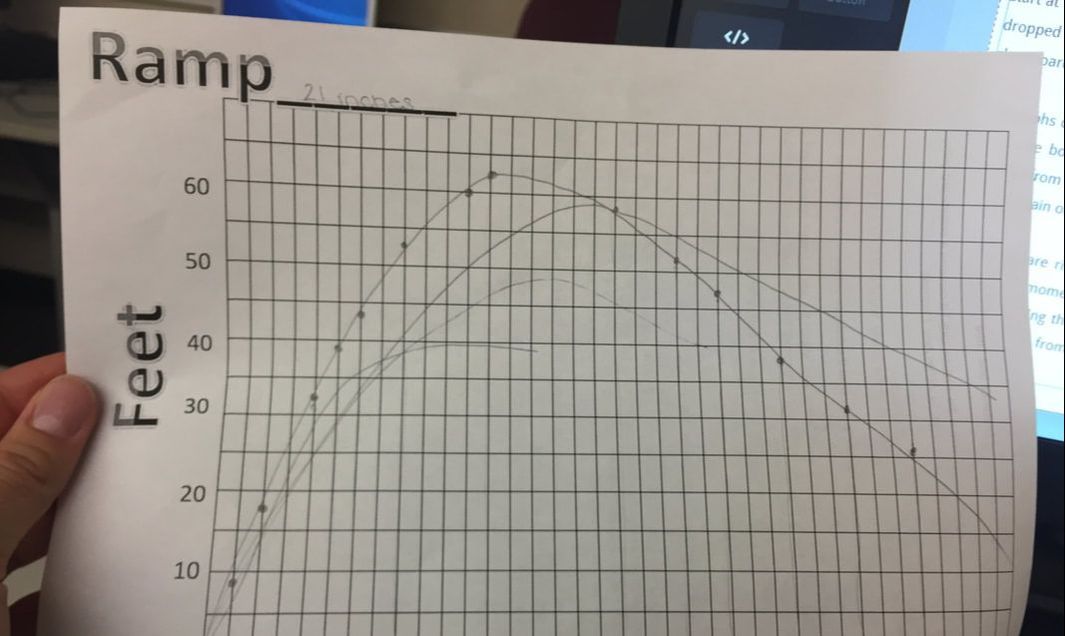 This is the graph for the skateboard that was dropped from the 21 inch ramp. As you can see, the maximum distance traveled of this skateboard was about 63 feet. 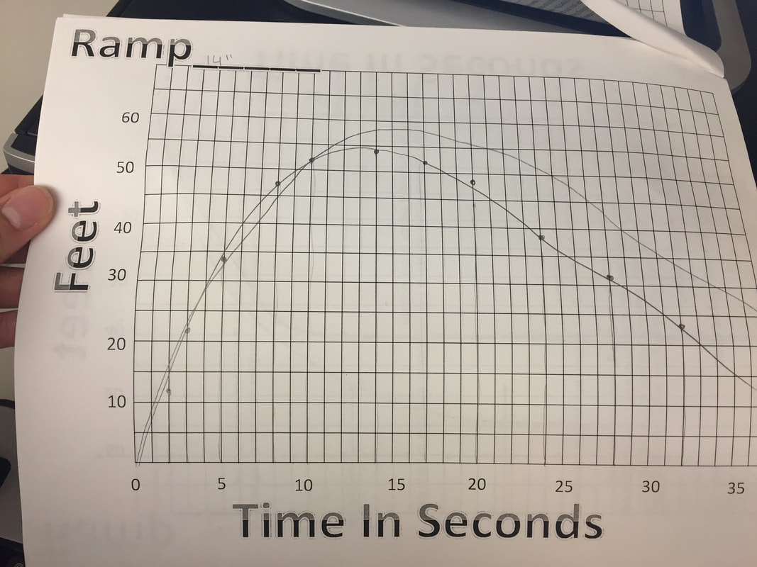 This is the graph for the skateboard that was dropped from the 14 inch ramp. The maximum of this graph is about 55 feet. 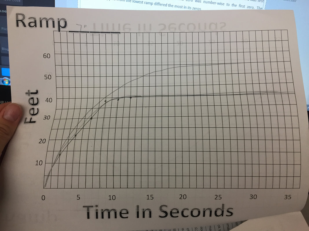 This is the graph for the skateboard that was dropped from the 7 inch ramp. This skateboard traveled a maximum distance of about 40 feet before leveling out.
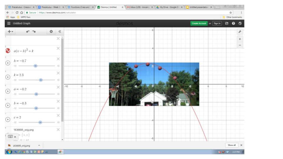 It appears to me that the ball will go into the hoop if some outside force does not deter its current direction. Due to the graph not touching each point, my calculated graph could be a little off in determining the end point of the ball.
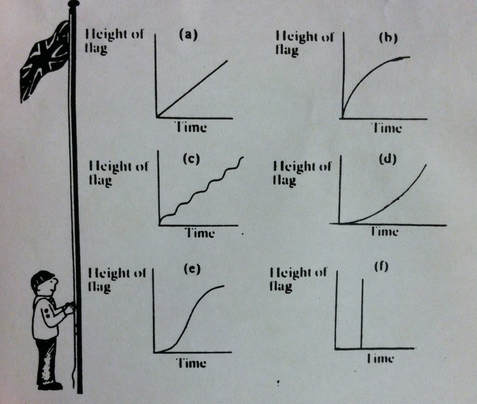 In graph A, the boy scout hoists the flag up at a constant speed without stopping for a break. In graph B, he hoists the flag at a quick pace at first, but then gradually slows as the flag gets higher. In graph C, the boy scout hoists the flag in consistently timed spurts, pausing for a brief moment in between but the flag is traveling at a constant speed when being raised. In graph D, the flag is being hoisted slowly as it first begins to go up, but as it gets higher its speed gradually increases. In graph E, he raises the flag slowly at first, then very quickly until the flag is near the top, where he slows again as the flag reaches its intended height. In the last graph, the boy scout waited to raise the flag until x minutes after he placed the flag on the pole, when he then raised the entire flag at a very fast, constant speed until it reached the top.
Graph C shows the situation most realistically, because the average person most likely would need to stop to adjust their hands after each length that the flag was raised. Graph F is the least realistic because the likelihood of a boy scout raising a flag at a constant speed without passing any time is probably close to none. |
Kayla CampbellArchives
November 2017
Categories |
 RSS Feed
